We can use auxiliary information in a variety of ways to improve estimates over SRS. In particular we note that since the most influential units in an estimate are often the largest, it is often in our interest to make sure we select the largest units with higher probability than the smaller units. This idea leads naturally to probability proportional to size sampling, where each unit has a distinct probability of selection \(\psi_i\) on any given draw, which is related to its size.
Let’s say we want to estimate the number of calves born in spring on farms supplying milk for Town Milk Supply. We have information on the number of milking cows on each such farm and indeed each cow is registered on a computer database. Farms vary in size, and we want to make sure we give larger farms (those with more cows) a greater chance of selection, since they will contribute more variability to our estimates. Assume that there are \(N\) farms, labelled \(i=1,\ldots,N\) , and that there are \(X_i\) cows on farm \(i\) .
We give farm \(i\) a probability of selection of \(\psi_i=X_i/X\) on each draw from the population. Here \(X=\sum_i X_i\) is the total number of cows on all the farms. We want to have a sample of \(n\) farms. To achieve this we put the \(N\) farms into a list, and then number all of the cows on all of the farms as \(1,\ldots,X\) .
There are \(X_1\) cows on the first farm, so they are numbered \(1,\ldots,X_1\) . On the second farm where there are \(X_2\) cows we number them \(X_1+1,\ldots,X_1+X_2\) . The cows on the third farm are numbered \(X_1+X_2+1,\ldots,X_1+X_2+X_3\) and so on up to the \(N^\) farm and the \(X^\) cow.
To choose our random sample we:
Note that this sampling is probability proportional to size with replacement (PPSWR). We don’t remove a farm (or a cow) from the list once it has been selected. This is necessary since there is no (known? possible?) way to select a probability proportional to size (PPS) sample without replacement. Inevitably, therefore, we will end up with some farms being selected more than once. What do we do with them? We do not drop the repeated observations – we must use the observations for those farms as many times as they appear.
We only collect the data once of course, it’s just that if a unit appears more than once in the sample, we must use its data repeatedly in our estimator.
An alternative way of drawing a PPSWR which is simpler to implement than the cumulative method given above is the Rejection Method. Here again we have \(N\) units in the population, and a size measure \(X_i\) for each one. The largest unit is of size \(M_X=(X_i)\)
This is called a rejection method, since sometimes we consider a unit for inclusion in the sample, but then reject it. In general it takes more than \(n\) passes through the sequence of steps to select \(n\) sample members.
Consider the following population of \(N=6\) university classes:
| Unit, \(i\) | Size, \(X_i\) | Cumulative size, \(_i=\sum_^iX_j\) |
|---|---|---|
| 1 | 10 | 10 |
| 2 | 15 | 25 |
| 3 | 40 | 65 |
| 4 | 40 | 105 |
| 5 | 80 | 185 |
| 6 | 100 | 285 |
We have a size measure for each unit \(X_i\) =the number of student in class \(i\) . We have calculated the cumulative running total \(_i\) of \(X_i\) for all units up to an including unit \(i\) . The total of the sizes is \(X=_N=285\) . Now let’s select a sample of size using the cumulative method. We generate four random numbers in the range \(1,\ldots,285\) : say these numbers are \(\\) . The \(165^\) student is in class 5, so we select that class into the sample. The \(205^\) student is in class 6, and so is the \(197^\) , so we select class 6 twice into the sample. Finally the \(12^\) student is in class 2. Thus our final sample is \(\\) .
How does the rejection method work in this situation? We first note that the largest class has size \(M_X=100\) . We select a random number \(i\) in the range \(1,\ldots,6\) , say \(i=4\) : thus we are considering class 4 for selection, which has size 40. We then draw another random number \(r\) in the range \(1,\ldots,100\) : say \(r=2\) . We see that \(r\leq X_4\) (i.e. \(2\leq 40\) ), so we select class 4 into the sample as the first unit.
Next we select another \(i\) value – say we get \(i=4\) again. We draw \(r\) again, but this time get \(r=99\) , which is greater than \(X_4=40\) . So we reject class 4 as the second unit.
We continue in this way, drawing pairs of random numbers \((i,r)\) and testing to see if \(r\leq X_i\) .
| \(i\) | \(r\) | \(X_i\) | \(r\leq X_i\) ? | Action |
|---|---|---|---|---|
| 4 | 2 | 40 | Yes | Acecpt class 4 |
| 4 | 99 | 40 | No | Reject and continue |
| 6 | 57 | 100 | Yes | Accept class 6 |
| 5 | 63 | 80 | Yes | Accept class 5 |
| 2 | 86 | 15 | No | Reject and continue |
| 2 | 57 | 15 | No | Reject and continue |
| 6 | 33 | 100 | Yes | Accept class 6 |
So we end up with the sample \(\\) .
We have seen that the probability that a unit is selected on any given PPSWR draw is \(\psi_i=X_i/X\) . What is the probability \(\pi_i\) that a unit is selected into sample of size \(n\) ?
The probability that a unit is selected is one minus the probability that on every one of the \(n\) draws it is not selected: \[\begin \pi_i = 1 - (1-\psi_i)^n = 1-\left(1-\frac\right)^n \tag \end\] By noting that \[\begin p(\text) &=& p(i) + p(j) - p(\text)\\ &=& p(i) + p(j) - [1-p(\text)] \end\] it can easily be shown that the 2nd order inclusion probabilities are: \[\begin \pi_ = 1-(1-\psi_i)^n-(1-\psi_j)^n+(1-\psi_i-\psi_j)^n \end\]
We have already noted that in with replacement sampling, there is a chance that a unit may be selected multiple times. In general unit \(i\) is selected \(Q_i\) times, where \(Q_i\) is a Binomial random variable: \[\begin Q_i \sim (n,\psi_i) \end\] and the full set of \(N\) \(Q_i\) values is distributed according to a multinomial distribution \[\begin \sim (n,\psi) \end\]
The Horwitz-Thompson estimator of the total is, as always \[\begin \widehat = \sum_
The question as to whether the HH estimator or the HT estimator has the smaller variance is not straightforward and in fact depends on the particular configuration of the population values: how correlated are the variable of interest and the size measure, what are the coefficients of variation of the variable of interest and the size measure, etc.
The Hansen-Hurwitz estimator of the mean follows straightforwardly from that for the total: \[\begin \widehat>_ = \frac_> = \frac \sum_ \frac <\psi_k>\end\] This estimator is unbiased and has variance \[\begin \bfa<\widehat>_> = \frac\sum_^\left(\frac><\psi_i>-Y\right)^\psi_ \end\] which can be estimated from the sample by \[\begin \bfa<\widehat>_> = \frac \sum_\left(\frac<\psi_k>-\widehat_\right)^ \end\]
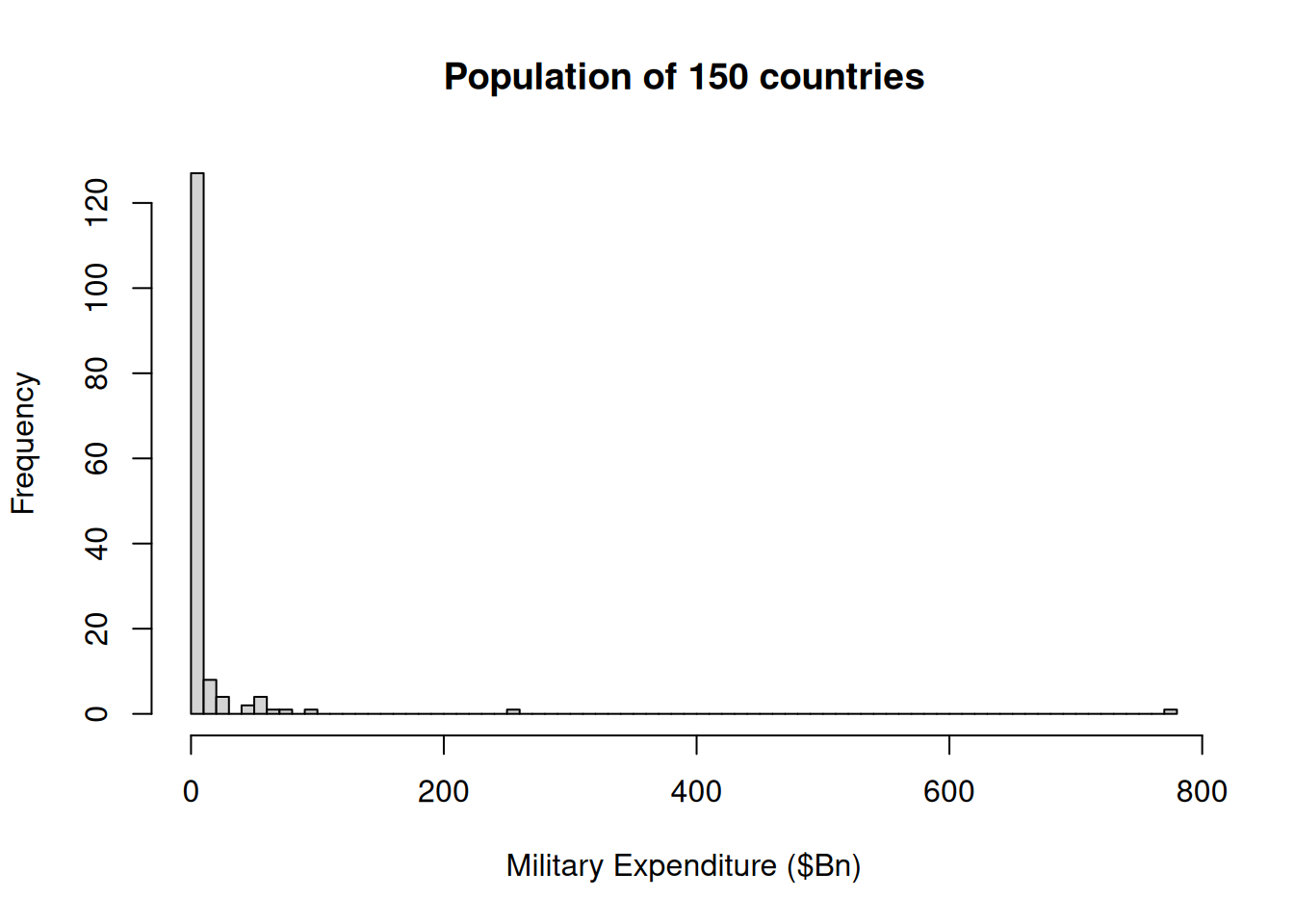
We have a dataset of the 2020 population, GDP and military expenditure of \(N=150\) countries.
## [1] 150
Figure 7.1: 2020 Military Expenditure
The distribution is very strongly right skewed - with the USA dominating expenditure. The total value of all military expenditure in 2020 was Bn$2000.07
If we take a SRSWOR of \(n=30\) countries we can create an estimate of the total world military expenditure.
The data in the sample are listed in Table 7.3 and displayed in Figure 7.2.
| Country | Population | GDP (Bn$) | Military Expenditure (Bn$) |
|---|---|---|---|
| Angola | 32866268 | 104.128681 | 0.9935944 |
| Belarus | 9379952 | 58.482353 | 0.8445129 |
| Brazil | 212559409 | 1749.104722 | 19.7363478 |
| Canada | 38005238 | 1600.331195 | 22.7548471 |
| Central African Republic | 4829764 | 2.001438 | 0.0413036 |
| Congo, Dem. Rep. | 89561404 | 45.259707 | 0.3620916 |
| Gambia, The | 2416664 | 1.672833 | 0.0148050 |
| Ghana | 31072945 | 62.724595 | 0.2398872 |
| Guinea-Bissau | 1967998 | 1.218760 | 0.0233067 |
| Haiti | 11402533 | 14.956795 | 0.0002638 |
| Iraq | 40222503 | 170.857728 | 7.0155588 |
| Italy | 59554023 | 1744.731952 | 28.9213428 |
| Jamaica | 2961161 | 13.440715 | 0.2444328 |
| Korea, Rep. | 51780579 | 1623.895081 | 45.7353926 |
| Kosovo | 1775378 | 7.144368 | 0.0789650 |
| Liberia | 5057677 | 3.115543 | 0.0169370 |
| Malta | 525285 | 12.886270 | 0.0806132 |
| Moldova | 2620495 | 8.517410 | 0.0445338 |
| Montenegro | 621306 | 4.046328 | 0.1020905 |
| Morocco | 36910558 | 105.726172 | 4.8309564 |
| Mozambique | 31255435 | 17.959222 | 0.1537419 |
| Norway | 5379475 | 403.779725 | 7.1125385 |
| Paraguay | 7132530 | 40.446809 | 0.3643422 |
| Peru | 32971846 | 190.979129 | 2.6331234 |
| Romania | 19286123 | 208.838847 | 5.7268442 |
| Slovenia | 2100126 | 48.124693 | 0.5748319 |
| Somalia | 15893219 | 5.151914 | 0.0983850 |
| Tunisia | 11818618 | 44.681504 | 1.1573724 |
| Turkey | 84339067 | 1015.326663 | 17.7246321 |
| Zambia | 18383956 | 23.418946 | 0.2121424 |
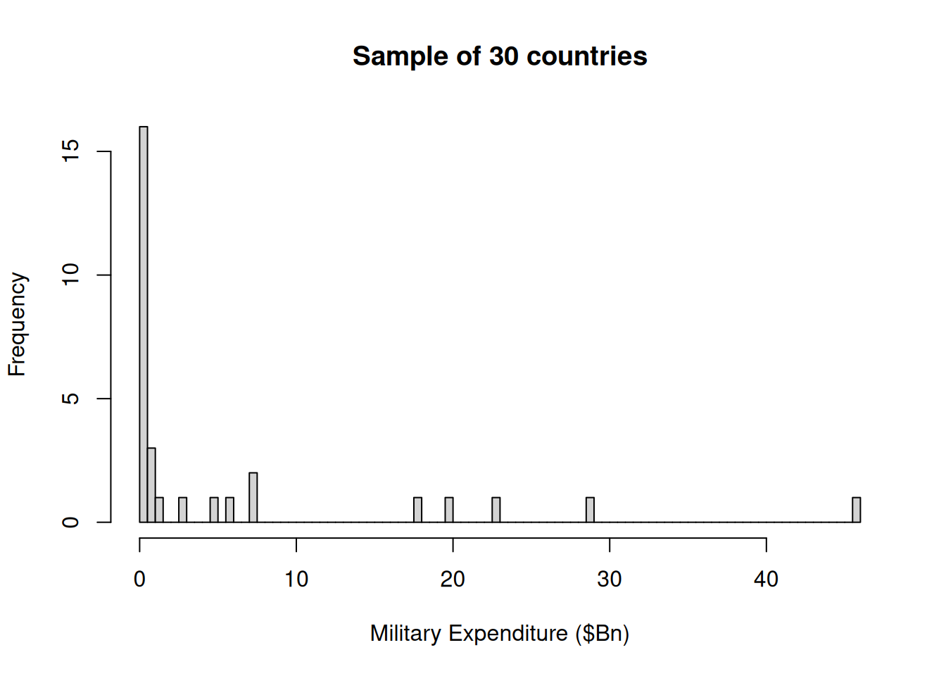
Figure 7.2: Military Expenditure of a SRSWOR of 30 countries
The mean expenditure in the sample is Bn$5.59 with standard deviation Bn$10.79. This leads to an estimate of \[ \widehat_ = N\bar = (158)(5.59) = 839.2 \] with standard error \[\begin \bfa<\widehat_> &=& \sqrt
In a situation where we have a variable on the frame that is likely to correlate with the size of military expenditure, we can use PPSWR to do a lot better. Gross Domestic Product (GDP) does correlate strongly with military expenditure - as can be seen in the diagram below.
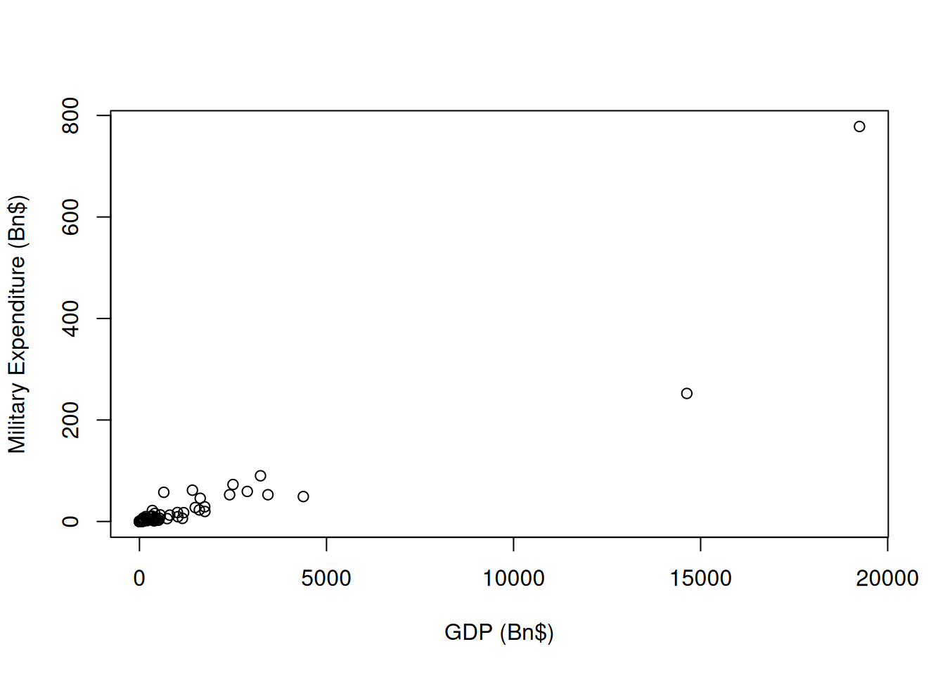
Figure 7.3: GDP and Military Expenditure
Note that we could use population size, but GDP is a better indicator of the size of the economy, which is what we would expect to correlate best with military expenditure).
If we select a sample of \(n=30\) countries by ppswr we get, for example, the units
8, 8, 11, 13, 31, 31, 31, 31, 31, 50, 50, 54, 65, 65, 73, 77, 98, 103, 133, 134, 147, 148, 148, 148, 148, 148, 148, 148, 148, 150
There are a few units which have been selected multiple times – most notably Unit 31 (China) and Unit 148 (USA), which respectively occur 5 and 8 times out of 30.
An estimate of the population total from this sample is \[\begin \widehat_ &=& \frac \sum_ \frac <\psi_k>\\ &=& 2032.41 \end\] This is a very good estimate (recall that the true value is 2000.07).
If we are carrying out a simple random sample with replacement (SRSWR), the probability a unit is selected on each draw is the same for every unit: \[ \psi_i= \frac \] So the HH estimator of the population total from a SRSWR of size \(n\) is \[\begin \widehat_ &=& \frac\sum_^n \frac<\psi_k>\\ &=& \frac\sum_^n y_k\\ &=& N\bar \end\] which is exactly the same as the HT estimator from SRSWOR. The weights are just the same: \(w_k=N/n\) .
However the variance estimator is different: \[\begin \bfa>_> &=& \frac \sum_^n \left(\frac <\psi_k>- \widehat_\right)^2\\ &=& \frac \sum_^n \left(Ny_k - N\bar\right)^2\\ &=& \frac \sum_^n \left(y_k - \bar\right)^2\\ &=& N^2\frac \end\] which is almost the same as the HT estimator: except that it lacks the finite population correction: \[\begin \bfa>_> &=& N^2\left(1-\frac\right)\frac \end\] This means that even as \(n\rightarrow N\) the variance of the estimator does not decrease to zero. That’s because is a with-replacement design, a sample of size \(n=N\) is not guaranteed to be a census.
That makes the variance of the SRSWR estimator a bit larger than that of the SRSWOR design – and the estimator is less efficient. i.e. for the same sample size \(n\) we get a larger variance.
The lack of efficiency due to the lack of the fpc is typical of with-replacement designs. However if \(n\) is much smaller than \(N\) the loss of efficiency isn’t important.
In PPSWR designs where the size measure \(X_i\) is strongly correlated with the characteristic of interest \(Y_i\) then (even without the fpc) PPSWR can have dramatic gains over SRSWOR.
Also note that if the fpc is ignored in any survey sampling analysis (and it often is) – then the analysis effectively treats the sampling as if it were with replacement. Moreover, if we are given data from a complex design – but are only given the survey weights (without enough information to calculate the joint selection probabilities) then we are forced into treating the sample as if it were drawn with replacement.